Power BI:
Conditional formatting is a feature in Power BI and Excel that enables us to use gradient colors to define customized cell colors based on cell values, other values, or fields.
A new ‘Icon’ feature is available for conditional formatting in Power BI. In this article you will learn how to perform conditional formatting by icons.
Follow the below step to apply conditional formatting by ‘Icon’.
Step 1 :
Import your data in Power BI. I am importing an Excel file Go to ‘Get data’ at home tab and click on ‘Excel’. Provide file path and click on ‘Open’
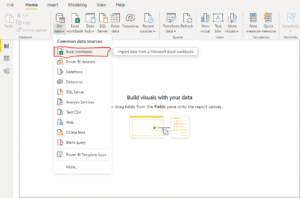
Table will be shown at the right pane of the Power BI desktop tool. I marked it red in the below image.
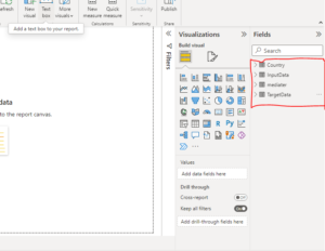
Setp 2 :
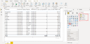
To show table data use table visualization. For applying conditional formatting, Table and Matrix visualization is a good choice. Go to visualization and click on table visual, also check the columns of the table that you want to show in the table.
The selected columns with yellow check box in the below image and table visualization are highlighted in the visualizations panel.
Step 3 :
Select any column from values on which you want to apply conditional formatting. I am selecting Quantity column; i.e. ‘sum of quantity’.
To access conditional formatting, pick the down arrow next to the value in the Values well that you want to format in the Visualizations pane in Power BI Desktop in the Fields well (or right-click the field). In the Values area of the Fields area, you can only handle conditional formatting for fields. See the below image.
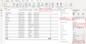
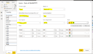
Once you click on ‘Icons’ a new Window will be opened. In ‘Style’ you can choose any style.
Provide all required filed values and click on ‘Ok’ to apply.
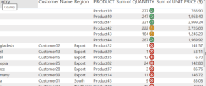
The icons that you choose will be shown at right to the ‘Quantity’ values. See the below image.
https://www.crmonce.com/automatically-creates-pass-workers-status-approved/
For any Help or Queries Contact us on info@crmonce.com or +918096556344

